The Regression-Discontinuity Design
In this exercise you are going to create data for a regression-discontinuity design. It can be depicted in notational form as:
where each O indicates an observation or measure on a group of people, the X indicates the implementation of some treatment or program, separate lines are used to depict the two groups in the study, the C indicates that assignment to either the treatment or control group is done using a cutoff score on the pretest assignment measure, and the passage of time is indicated by moving from left to right. We will assume that we are comparing a program and comparison group (rather than a relative comparison of two programs or different levels of the same program).
The regression-discontinuity design is a type of nonequivalent group design that is characterized by its method of assigning persons to groups using a cutoff score on an assignment measure — all persons who score above the cutoff are assigned to one group while those scoring on the other side are assigned to the other. Two things need to be decided when selecting a cutoff value. First we need to decide whether the high or low pretest scorers will receive the program. We might give the program to the high pretest scorers if we are studying the effects of scholarships (high achievement), awards (high performance), novel medical treatments or therapies (high on measures of illness) and so on. We might give the program to the low pretest scorers when studying compensatory education (low achievement), poverty (low income), and so on. In this exercise we will simulate a program given to the low pretest scorers. Second, we need to decide the specific value of the pretest cutoff. In the real world, cutoff values are selected in a number of ways. When there are a limited number of program openings, the cutoff score can be selected so that exactly the desired number of persons score either above or below it (depending on whether the program goes to high or low scorers). In other situations, some theoretical value is appropriate for the cutoff. For example, the pretest average might be chosen as the cutoff because in a particular context it makes sense to give the program to those who are "below average" or "above average". In this exercise we arbitrarily use a cutoff equal to the theoretical pretest average.
You will again make use of the pretest and posttest scores that you generated in the first exercise. If you recall that the pretest scores (as generated in the first exercise) can range from 4 to 24, it should be clear that the expected pretest average is 14 units. Thus, we will assign all cases having a pretest score less than or equal to 14 units to the program group and all others to the comparison group (remember that in this simulation the program is given to the low pretest scorers). The assignment strategy can be summarized as follows:
where Z is the 0,1 "dummy" assignment variable.
You will generate the data for this exercise using Table 4-1. In the first column of Table 4-1 you should copy the pretest scores (Table 1-1, column 5) from the first exercise into column 2 of Table 4-1. Now, examine the pretest score for person 1. If it is less than or equal to 14, enter a '1' in Column 3 of Table 4-1 labeled Group Assignment (Z). If it is 15 or higher, enter a '0'. Continue doing this for all 50 persons. When you have finished, notice that the next column, labeled "Hypothetical Program Effect" consists entirely of '7's, that is, the program will increase the posttest scores of each program participant by 7 units. But not everyone gets the program and so not everyone should get the effect of 7 units. You only want those persons who have a Z = 1 (program persons) to get the 7.
An easy way to accomplish this is to multiply the assignment variable (Column 3) by the effect size (Column 4) and put the result in Column 5, labeled "Effect of Program". So, the fourth column should have '7's for all program persons and '0's for all comparison group persons. Next, you should copy the posttest scores from the first exercise (Column 6 of Table 1-1) into column 6 of Table 4-1. Finally, to get the posttest scores with the program effect included you simply add the "Effect of Program" (Column 5) and posttest scores (Column 6) and place the result in Column 7 of Table 4-1 labeled "Posttest (Y) for Regression-Discontinuity Design."
It is useful at this point to stop and consider what you have done. In the first exercise you generated the pretest according to
X = T + eX
and in this exercise you constructed the program assignment variable Z using a cutoff rule. Then, using a hypothetical program effect of G = 7 units (G for Gain), you constructed the effect of the program by multiplying GZ. You then copied the posttest from the first exercise and you should recall that it was generated by the model:
Y = T + eY
Finally, you added the effect of the program to this posttest value and obtained the posttest for this exercise:
Y = T + GZ + eY
Again, it is always important to examine the data visually and so you should graph the univariate pretest distribution in Figure 4-1 and the univariate posttest distribution in Figure 4-2. As in previous exercises, be sure to use a different colored pen or pencil for the program and comparison groups. Also, estimate the central tendency for each group on both graphs using either the counting method or by computing the averages. You should also graph the bivariate distribution as you did before, remembering to keep the marks for the two groups distinct both in color and symbol. Also, estimate the line that fits through the bivariate data.
Let's consider the univariate distributions. Clearly, the pretest distribution in this exercise is identical to the pretest distribution of the first exercise. The only difference is that the program group has scores of 14 or less and the comparison group has scores of 15 or more. Notice that because of this the pretest averages for the two groups are very different. This is what we mean when we say that the regression-discontinuity design induces maximal pretest differences between the groups. Now look at the posttest distribution. If this was all the information you had (i.e., you did not know the pretest information) you would probably conclude that the program and comparison groups don't differ much — that is, the program is not effective. It is only when you consider how different they are on the pretest that you can see there is a program effect, that is, the program group did much better than would have been expected on the basis of their pretest scores.
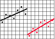
Next, look at the bivariate distribution. As in the previous exercise, you visually fit separate lines for the program and comparison groups. Let's use these jagged lines to try to estimate a straight line that fits through the data. You will have to do this visually. The figure below shows the dots estimated in each column from a hypothetical example and the lines connecting them. It also shows the straight line that we visually estimated to fit through the jagged one. You should estimate the line for the program and comparison groups separately. The program group line should be to the left of column 14 (and include it) and the comparison group one should be to the right.
You can easily estimate the slopes of these lines. First, take the program group line. Place a dot somewhere on this line at a point where one of the column lines intersects the straight line. Now move exactly two columns to the right and place a dot where the straight line intersects the column line. At this point, you should have something that resembles the following:
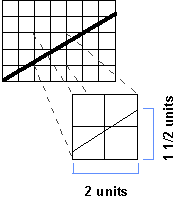
You know that the horizontal line is exactly 2 units wide. Measure the vertical distance between the two dots in your graph. Be sure that you measure this distance in terms of the units of the graph. Let's say that you find that it is about 1⅓ units high. To estimate the slope, you simply construct a ratio where the vertical distance is the numerator and the horizontal distance is the denominator. In this example, you would calculate:
slope = (1½) / 2
= 1.5 / 2
= .75 or ¾
The slope enables us to say how much change in the vertical direction we get for each 1-unit change in the horizontal direction. In this example, for every increase of 1 unit in the X direction we get an increase of .75 units or ¾ unit in the Y direction. The estimates of slope for the program and comparison group lines should be very similar.
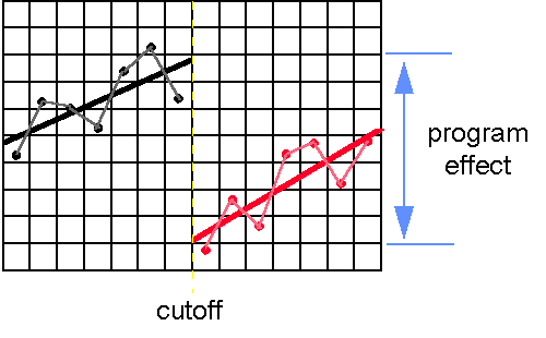
Now let's estimate the size of the program effect. First, draw a vertical line through the entire bivariate distribution at the cutoff point (i.e., X = 14). Place a dot where the program group straight line intersects the cutoff line. Similarly, place a dot where the comparison group line intersects the cutoff line. Now count the number of vertical units between these two dots. This is the regression-discontinuity estimate of the program effect. You should find that this estimate is about 7 units which is, of course, what you put in. This is illustrated in the figure below.
After completing the previous exercise, you should be convinced of the following: Although in these dice rolling simulations we have avoided presenting statistical terminology as much as possible, our discussion of the regression-discontinuity design would not be complete without it. After all, the first half of the name of this design is "regression." It should be no surprise that when we statistically analyze this design in the real world, we use regression analysis. Here, we consider some of the major issues involved in such an analysis.
A crucial step in the analysis of data from the regression-discontinuity design involves guessing the true shape of the regression line. In our example this is easy to do because we created the data and we know that the true shape is a straight line in each group. This is because the pretest and posttest both share the same true score. In real life, we don't often know what the true regression shape is, and we have to guess at it. Thus, if you were conducting a real data analysis, you might try a variety of regression lines until you were confident that you had captured this true shape.
Since we know that the true shape in this case is linear, we could construct the appropriate regression model as follows:
Y = b0 + b1X* + b2Z + eY
where:
Y = the posttest
X* = the pretest minus the cutoff value (i.e., X − 14)
Z = the 0,1 group assignment variable
b0 = the intercept, that is, the y value at which the comparison group regression line meets the cutoff line
b1 = the slope (we assume it's the same in both groups)
b2 = the program effect, that is, the amount you must add or subtract to b0 in order to find where the program group regression line meets the cutoff line
eY = random error
In regression-discontinuity analysis, we usually subtract the cutoff value from each pretest score before the analysis so that the cutoff is at a value of X = 0 which is the intercept in the model. Notice that the term b2Z is simply the program effect b2 times the assignment variable (Z) which is exactly what we put in as GZ. You should be able to estimate all of the b's in the formula above from the bivariate graph. First, b0, is the posttest value for the point you marked on the cutoff line where the comparison group line intercepts it. Second, b1, is the estimate of the slope. If your program and comparison group slope estimates differed considerably take the average of the two. Finally, b2, is the program effect — the posttest (Y) distance between the two regression lines at the cutoff. Let's say that you estimate b0 = 14, b1 = .5 and b2 = 7. You could then write out the regression formula as:
Y = 14 + .5X* + 7Z
(We drop the eY term out because that describes deviations from the regression lines.) Basically, when you run a regression-discontinuity analysis you enter in the values for Y, X* (remember to subtract the cutoff from each X) and Z and the regression program gives you the estimates of b0, b1, and b2.
You should be convinced that this single formula describes the regression lines for both groups as well as the program effect. To see this, you can construct the formula for each regression line separately. First, construct the formula for the program group line (substituting your own estimates instead of these) by setting Z = 1 (remember this is the program group):
YP = 14 + .5X* + 7(1)
YP = 14 + .5X* + 7
YP = 21 + .5X*
Now you can construct the formula for the comparison group line by substituting Z = 0.
YC = 14 + .5X* + 7(0)
YC = 14 + .5X*
Now, to convince yourself that the program effect is correctly estimated, construct the program effect at the cutoff. Remember that we subtracted the cutoff from each pretest value and so the cutoff is at X* = 0. Therefore, the Y estimate for the program group value at the cutoff in this example would be
YP = 21 + .5(0)
YP = 21
and the comparison group y value at the cutoff would be
YC = 14 + .5(0)
YC = 14
and, therefore, the program effect would be the difference between the two groups or
YP − YC = 21 − 14
YP − YC = 7
You should get a value close to the value of 7 units which is, of course, what you put in when you constructed the data. It should also be clear that when a dichotomous dummy variable (e.g., Z) is used in a regression equation, you are essentially telling the analysis that you want to fit two lines, one for each group having each value of Z.
Regression-Discontinuity Design — Table 4-1
| Person | Pretest X from Table 1-1 |
Group Assignment Z |
Hypothetical Program Effect |
Effect of Program |
Posttest Y from Table 1-1 |
Posttest (Y) for Regression-Discontinuity Design |
|---|---|---|---|---|---|---|
| 1 | 7 | |||||
| 2 | 7 | |||||
| 3 | 7 | |||||
| 4 | 7 | |||||
| 5 | 7 | |||||
| 6 | 7 | |||||
| 7 | 7 | |||||
| 8 | 7 | |||||
| 9 | 7 | |||||
| 10 | 7 | |||||
| 11 | 7 | |||||
| 12 | 7 | |||||
| 13 | 7 | |||||
| 14 | 7 | |||||
| 15 | 7 | |||||
| 16 | 7 | |||||
| 17 | 7 | |||||
| 18 | 7 | |||||
| 19 | 7 | |||||
| 20 | 7 | |||||
| 21 | 7 | |||||
| 22 | 7 | |||||
| 23 | 7 | |||||
| 24 | 7 | |||||
| 25 | 7 | |||||
| 26 | 7 | |||||
| 27 | 7 | |||||
| 28 | 7 | |||||
| 29 | 7 | |||||
| 30 | 7 | |||||
| 31 | 7 | |||||
| 32 | 7 | |||||
| 33 | 7 | |||||
| 34 | 7 | |||||
| 35 | 7 | |||||
| 36 | 7 | |||||
| 37 | 7 | |||||
| 38 | 7 | |||||
| 39 | 7 | |||||
| 40 | 7 | |||||
| 41 | 7 | |||||
| 42 | 7 | |||||
| 43 | 7 | |||||
| 44 | 7 | |||||
| 45 | 7 | |||||
| 46 | 7 | |||||
| 47 | 7 | |||||
| 48 | 7 | |||||
| 49 | 7 | |||||
| 50 | 7 |
Regression-Discontinuity Design — Figure 4-1
Regression-Discontinuity Design — Figure 4-2
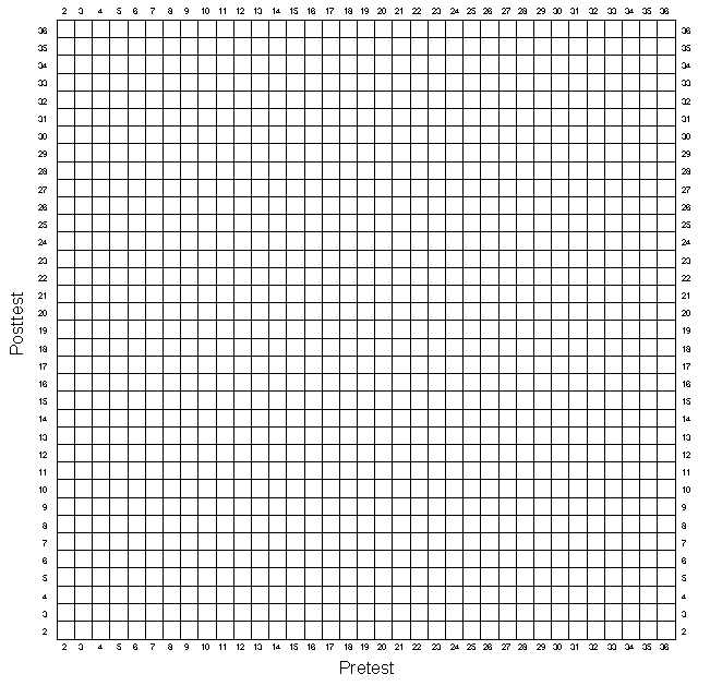
Regression-Discontinuity Design — Figure 4-3
